| time | status |
|---|---|
| 2 | 1 |
| 72 | 0 |
| 51 | 1 |
| 60 | 0 |
| 33 | 1 |
| 27 | 1 |
| 14 | 1 |
| 24 | 1 |
| 4 | 1 |
| 21 | 0 |
Chapter 4
(AST305) Lifetime Data Analysis I
4 Inference procedures for parametric models
Introduction
Likelihood methods for lifetime data were introduced in Chapter 2, which includes derivation of likelihood function for different types of censored data
Maximum likelihood estimator
Inference about parameters (hypothesis testing and confidence intervals)
Likelihood function (Complete data)
Let \(t_1, \ldots, t_n\) be a random sample from a distribution \(f(t; \boldsymbol{\theta})\), where \(\boldsymbol{\theta}\) is a \(p\)-dimensional vector of parameters
Likelihood and log-likelihood function \[\begin{aligned} L(\boldsymbol{\theta}) &= \prod_{i=1}^n f(t_i; \boldsymbol\theta)\\ \ell(\boldsymbol{\theta}) = \log L(\boldsymbol{\theta})& = \sum_{i=1}^n \log f(t_i;\boldsymbol{\theta}) \end{aligned}\]
Maximum likelihood estimator (MLE) \[\begin{align} \hat{\boldsymbol{\theta}} = {\arg\,\max}_{\boldsymbol{\theta} \in \Theta} \ell(\boldsymbol{\theta}) \end{align}\]
Statistical inference (Complete data)
Large sample property of MLE \[\begin{align} \hat{\boldsymbol{\theta}}\sim \mathcal{N}\big(\boldsymbol{\theta}, [\mathcal{I}(\boldsymbol{\theta})]^{-1}\big) \end{align}\]
Fisher expected information matrix \[\begin{align} \mathcal{I}(\boldsymbol{\theta}) = E\Big[-\frac{\partial^2\ell(\boldsymbol{\theta})}{\partial\boldsymbol{\theta}\,\partial\boldsymbol{\theta}'}\Big] \end{align}\]
Observed information matrix \[\begin{align} {I}(\hat{\boldsymbol{\theta}}) = -\frac{\partial^2\ell(\boldsymbol{\theta})}{\partial\boldsymbol{\theta}\,\partial\boldsymbol{\theta}'}\bigg\vert_{\boldsymbol{\theta} = \hat{\boldsymbol{\theta}}} \end{align}\]
Likelihood function (Type I or random censoring)
Data: \(\{(t_i, \delta_i),\;i = 1, \ldots, n\}\)
\(t_i\) is a sample realization of \(\tilde{T}_i=\min(T_i, C_i)\)
lifetime \(T_i\) follows a distribution with pdf \(f(t_i; \boldsymbol{\theta})\) and the corresponding survivor function \(S(t_i; \boldsymbol{\theta})\)
censoring time \(C_i\) could be random or fixed depending on the censoring mechanism
\(\delta_i = I(T_i \leq C_i)\), censoring indicator
Data for type I or random censoring \[\big\{(t_i, \delta_i),\;i = 1, \ldots, n\big\}\]
Likelihood function \[\begin{align} L(\boldsymbol{\theta}) & = \prod_{i=1}^n \big[f(t_i;\boldsymbol{\theta})\big]^{\delta_i}\,\big[S(t_i; \boldsymbol{\theta})\big]^{1- \delta_i}\notag \\ & = \prod_{i=1}^n \big[S(t_i;\boldsymbol{\theta})\,h(t_i; \boldsymbol{\theta})\big]^{\delta_i}\,\big[S(t_i; \boldsymbol{\theta})\big]^{1- \delta_i}\notag \\ &= \prod_{i=1}^n \big[S(t_i;\boldsymbol{\theta})\big]\,\big[h(t_i; \boldsymbol{\theta})\big]^{\delta_i} \end{align}\]
Likelihood function (Type II censoring)
Let lifetime \(T_i\) \((i=1, \ldots, n)\) follows a distribution with pdf \(f(t_i; \boldsymbol{\theta})\) and the corresponding survivor function \(S(t_i; \boldsymbol{\theta})\)
The experiment was terminated after observing \(r\) smallest lifetimes
\[ t_{(1)} \leqslant \cdots \leqslant t_{(r)} \]The remaining \((n-r)\) observations are considered as censored at \(t_{(r)}\)
Likelihood function \[\begin{align} L(\boldsymbol{\theta}) = \bigg[\prod_{i=1}^r f(t_{(i)}; \boldsymbol{\theta})\bigg]\,\Big[S(t_{(r)}; \boldsymbol{\theta})\Big]^{n-r} \end{align}\]
Statistical inference (censored sample)
For censored samples, the result “asymptotic distribution of MLE is normal” is still valid
The expression of the Fisher expected information matrix \(\mathcal{I}(\boldsymbol{\theta})\) is complex for censored data, observed information matrix \(I(\hat\theta)\) is used in making inference with censored sample
4.1 Exponential Distribution
The exponential distribution is the first lifetime model for which statistical methodology were extensively developed
Exact tests can be developed for exponential distribution for certain type of censoring mechanism
Exponential distribution assume constant hazard and its use is limited for analyzing real life problems
Probability density function \[ f(t; \theta) = (1/\theta)\,\exp({-t/\theta}) \quad \quad t\geqslant 0,\;\theta>0 \]
Hazard function \[ h(t; \theta) = (1/\theta) \]
Survivor function \[ S(t; \theta) = \exp(-t/\theta) \]
\(p\)th quantile \[ S(t_p;\theta) = 1 - p \;\;{\color{purple}\Rightarrow}\;\; \exp(-t_p/\theta) = 1- p \;{\color{purple}\Rightarrow}\; {\color{blue}t_p = -\theta\log(1-p)} \]
Homework
- Estimation and related inference of exponential distribution when the sample has no censored observations
Type I or random censoring
Lifetime \(T\sim \text{Exp}(\theta)\), \(\theta>0\)
Data: \(\big\{(t_i, \delta_i), i=1, \ldots, n\big\}\)
Likelihood function \[\begin{align} L(\theta) & = \prod_{i=1}^n \big[f(t_i; \theta)\big]^{\delta_i}\,\big[S(t_i;\theta)\big]^{1-\delta_i} \notag \\ &= \prod_{i=1}^n S(t_i;\theta) \,\big[h(t_i;\theta)\big]^{\delta_i} \notag \\ & = \prod_{i=1}^n \exp(-t_i/\theta)\,(1/\theta)^{\delta_i} \end{align}\]
Likelihood function \[\begin{align} L(\theta) & = \prod_{i=1}^n \exp(-t_i/\theta)\,(1/\theta)^{\delta_i}\notag \end{align}\]
Log-likelihood function \[\begin{align} \ell(\theta) & = \sum_{i=1}^n\big[-(t_i/\theta) - \delta_i\log(\theta)\big] \notag \\ & = -\frac{1}{\theta} \sum_i t_i -r \log (\theta) \end{align}\]
- \(r = \sum_i \delta_i\;\rightarrow\) the number of failures observed in the sample
Log-likelihood function \[\begin{align} \ell(\theta) & = -\frac{1}{\theta} \sum_i t_i -r \log (\theta)\notag \end{align}\]
MLE \[ \frac{\partial\ell(\theta)}{\partial\theta}\Bigg\vert_{\theta=\hat{\theta}} =0 \;\;{\color{purple}\Rightarrow}\;\; \frac{1}{\hat\theta^2}\sum_i t_i - \frac{r}{\hat\theta} = 0 \] \[\begin{align} {\color{purple} \hat\theta = \sum_{i=1}^n t_i/r} \end{align}\]
- Assuming \(r>0\) and no finite MLE exists for \(r = 0\)
- Information matrix
\[\begin{align} I(\theta) &= -\frac{\partial^2\ell(\theta)}{\partial\theta^2} \notag \\ & = -\frac{\partial}{\partial\theta}\Bigg[\frac{1}{\theta^2}\sum_i t_i - \frac{r}{\theta}\Bigg] \notag \\ & = \frac{2}{\theta^3} \sum_i t_i - \frac{r}{\theta^2} \end{align}\]
- Replacing the parameter \(\theta\) by its MLE \(\hat\theta = \sum_i t_i/r\), the observed information matrix becomes \[ {\color{purple} I(\hat\theta) = \frac{r}{\hat{\theta}^2}} \]
Confidence interval (Method I)
Using \(\hat\theta\)’s asymptotic distribution \[\begin{align*} Z_1 = \frac{\theta - \hat\theta}{\big[I(\hat\theta)\big]^{-1/2}} = \frac{\theta - \hat\theta}{\hat\theta/\sqrt{r}} \sim \mathcal{N}(0, 1) \end{align*}\]
For a small sample, \(Z_1\) does not approximate the standard normal distribution very accurately
For a sample with a small number of uncensored observations, \(\ell(\theta)\) tends to be asymmetric
Confidence interval (Method II)
Sprott (1980) showed that \(\ell_1(\phi)=\ell(\phi^{-3})\) is more closer to symmetric compared to \(\ell(\theta)\), where \(\phi = \theta^{-1/3}\Rightarrow\,\phi^3=1/\theta\) \[\begin{align} \ell(\theta) & = -(1/\theta)\sum_i t_i - r\log \theta \\ {\color{purple}\ell_1(\phi)} &{\color{purple}= -\phi^3 \sum_i t_i + 3r \log (\phi)} \end{align}\]
MLE \(\;\;\;\;\;\hat\phi = \hat\theta^{-1/3} = \Big[{\sum_i t_i}/{r}\Big]^{-1/3}\)
Observed information matrix \[ \begin{aligned} I_1(\phi) = 6\phi \sum_i t_i + \frac{3r}{\phi^2} \;\;\Rightarrow\;\; {\color{purple}I_1(\hat\phi) = \frac{9r}{\hat\phi^2}} \end{aligned} \]
Pivotal quantity \[ Z_2 = \frac{\phi - \hat\phi}{\big[I_1(\hat\phi)\big]^{-1/2}} = \frac{\phi - \hat\phi}{\hat\phi/\sqrt{9r}} \sim \mathcal{N}(0, 1) \]
- Approximation of \(Z_2\) is quite accurate compared to that of \(Z_1\)
Confidence interval (Method III)
- Likelihood ratio statistic \(\Lambda(\theta)=2\ell(\hat\theta) - 2\ell(\theta)\) can also be used to obtain confidence interval for \(\theta\), where \[\begin{align} \ell(\theta) &= -(1/\theta)\sum_i t_i - r\log(\theta)\notag \\ & = -r(\hat\theta/\theta) - r\log(\theta) \\[.25em] \ell(\hat\theta) & = -(1/\hat\theta)\sum_i t_i - r\log(\hat\theta) \notag\\ & = -r - r\log(\hat\theta) \end{align}\]
LRT statistic \[ \begin{aligned} \Lambda(\theta) &= 2\ell(\hat\theta) - 2\ell(\theta) \\ & = 2r\big[(\hat\theta/\theta) - 1 + \log(\theta/\hat\theta)\big] \end{aligned} \]
Two-sided \((1-\alpha)100\%\) confidence intervals are obtained as the set of \(\theta\) values that satisfy \[\Lambda(\theta)\leq \chi^2_{(1), 1-\alpha}\]
Confidence interval of survivor function
Confidence interval for the parameter \(\theta\) can also be used to obtain confidence intervals for a monotone function of \(\theta\), such as \[ S(t; \theta) = \exp(-t/\theta) \;\;\text{or}\;\;h(t; \theta) = 1/\theta \]
Let \(100(1-\alpha)\%\) confidence interval for \(\theta\) \[ L(\text{Data}) \leqslant \theta \leqslant U(\text{Data}), \] where \(\text{Data}=\{(t_i, \delta_i), i=1, \ldots, n\}\)
- \(100(1-\alpha)\%\) confidence interval for \(S(t_0; \theta)=\exp(-t_0/\theta)\) \[ \begin{aligned} L(\text{Data}) &\leqslant \theta \leqslant U(\text{Data}) \\[.25em] t_0/U(\text{Data}) &\leqslant (t_0/\theta) \leqslant t_0/L(\text{Data}) \\[.25em] -t_0/L(\text{Data}) &\leqslant (-t_0/\theta) \leqslant -t_0/U(\text{Data}) \\[.25em] \exp\big(-t_0/L(\text{Data})\big) & \leqslant S(t_0; \theta)\leqslant \exp\big(-t_0/U(\text{Data})\big) \end{aligned} \]
Confidence interval of hazard function
- \(100(1-\alpha)\%\) confidence interval for \(h(t_0; \theta)=1/\theta\) \[ \big(1/U(\text{Data})\big) \leqslant h(t_0; \theta)\leqslant \big(1/L(\text{Data})\big) \]
Example 4.1.1
- Lifetimes (in days) of 10 pieces of equipment
- Assume lifetimes follow exponential distribution with parameter, i.e. \(T_i\sim \text{Exp}(\theta)\)
MLE \[ \hat\theta = \frac{\sum_i t_i}{r} = \frac{308}{7} = 44.0 \]
95% confidence interval of \(\theta\) (Method I)
\[\begin{align*} {\color{purple}\hat\theta \pm z_{.975}[I(\hat\theta)]^{-1/2}} &\;\;\Rightarrow\;\; \hat\theta \pm z_{.975}(\hat\theta/\sqrt{r})\\[.15em] &\;\; \Rightarrow\;\; 44.0 \pm (1.96)(44.0/\sqrt{7})\\[.15em] %&\;\; \Rightarrow\;\; 44.0 \pm 32.60\\ &\;\; \Rightarrow\;\; {\color{purple}11.4 \leqslant \theta \leqslant 76.6} \end{align*}\]
95% confidence interval of \(\theta\) (Method II)
\(\hat\phi = \hat\theta^{-1/3} = (44.0)^{-1/3} = 0.283\)
Confidence interval for \(\phi\)
\[ \begin{aligned} {\color{purple}\hat\phi \pm z_{.975}[I_1(\hat\phi)]^{-1/2}} &\;\;\Rightarrow\;\; \hat\phi \pm z_{.975}(\hat\phi/\sqrt{9r})\\[.15em] &\;\; \Rightarrow\;\; 0.28 \pm (1.96)(0.28/\sqrt{63})\\[.15em] %&\;\; \Rightarrow\;\; 0.28 \pm 0.07\\ &\;\; \Rightarrow\;\; {\color{purple}0.21 \leqslant \phi \leqslant 0.35} \end{aligned} \]Confidence interval for \(\theta\)
\[ \begin{aligned} {\color{purple}0.21 \leqslant \phi \leqslant 0.35} &\;\; \Rightarrow\;\; {0.21 \leqslant \theta^{-1/3} \leqslant 0.35} \\[.15em] &\;\; \Rightarrow\;\; {(0.35)^{-3} \leqslant \theta \leqslant (0.21)^{-3}} \\[.15em] &\;\; \Rightarrow\;\; {\color{purple}22.69 \leqslant \theta \leqslant 103.03} \end{aligned} \]
Likelihood ratio statistic \[ \Lambda(\theta) = 2r\big[(\hat\theta/\theta) - 1 - \log(\hat\theta/\theta) \big] \]
95% CI for \(\theta\) can be obtained from the set of \(\theta\)’s such that \[ \Lambda(\theta) \leq \chi_{(1), .95}^2 = 3.84 \]
95% CI for \(\theta\) \[ 22.8\;\; \text{to} \;\;102.4 \]
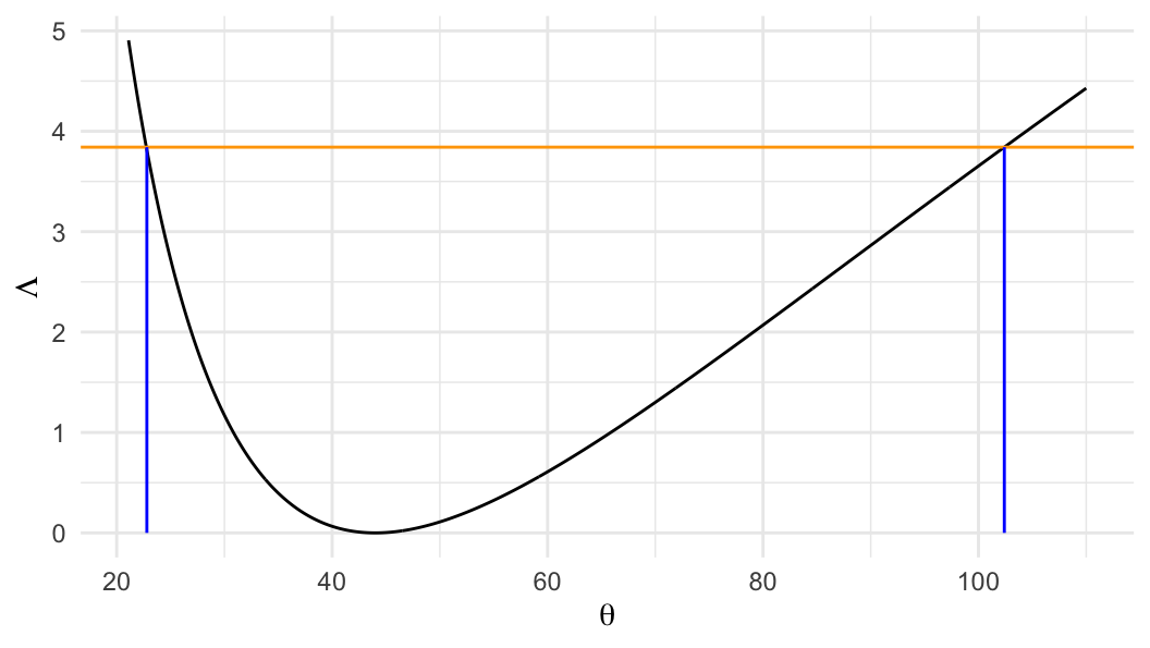
| method | lower | upper |
|---|---|---|
| Normal approx. | 11.40 | 76.60 |
| Sprott | 22.69 | 103.03 |
| LRT | 22.80 | 102.40 |
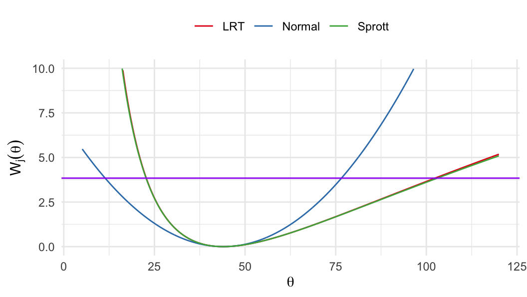
Methods for CI
Normal approximation \[ W_1(\theta) = \Bigg[\frac{(\hat\theta - \theta)}{\big[I(\hat{\theta})\big]^{-1/2}} \Bigg]^2 = (\hat\theta - \theta)^2 I(\hat\theta) \]
Sprott’s method \[ W_2(\theta) = \Bigg[\frac{(\hat\phi - \phi)}{\big[I_1(\hat{\phi})\big]^{-1/2}} \Bigg]^2 = (\hat\theta^{-1/3} - \theta^{-1/3})^2 I_1(\hat\theta^{-1/3}) \]
LRT \[ W_3(\theta) = 2\ell(\hat\theta) - 2\ell(\theta) = 2r\Big[(\hat\theta/\theta)-1-\log\big(\hat\theta/\theta\big)\Big] \]
\(W_j(\theta) \sim \chi^2_{(1)}\;\;j=1, 2, 3\;\;\text{under $H_0$}\)
Type II censoring plan
Assume lifetime \(T\sim\text{Exp}(\theta)\)
Let \(t_{(1)} < \cdots < t_{(r)}\) be the \(r\) smallest lifetimes observed from an experiment with \(n\;(\geq r)\) subjects
The joint distribution of \(t_{(1)}, \ldots, t_{(r)}\) \[\begin{align} f_T(t_{(1)}, \ldots, t_{(r)}) &= \frac{n!}{(n-r)!}\Big[\prod_{i=1}^r(1/\theta)e^{-t_{(i)}/\theta}\Big]\Big[e^{-t_{(r)}/\theta}\Big]^{n-r} \notag \\[.3em] & = \frac{n!}{(n-r)!} \;\big({1}/{\theta}\big)^r\;e^{-\frac{1}{\theta}\big[{\color{purple}\sum_{i=1}^r t_{(i)} + (n-r)t_{(r)}}\big]}\notag \\[.25em] & = \frac{n!}{(n-r)!} \;\big({1}/{\theta})^r \;e^{-{\color{purple}T_0}/\theta}\label{joint-type2} \end{align}\]
- The log-likelihood function \[\begin{align} \ell(\theta) &= -\frac{1}{\theta}\sum_it_{(i)} -r\log(\theta) - (1/\theta)(n-r)t_{(r)} +\text{Const.} \notag \\ & = -\frac{1}{\theta}\Big[\sum_{i=1}^r t_{(i)} + (n-r) t_{(r)} \Big] -r\log(\theta)+ \text{Const.} \notag \\ & = -\frac{T_0}{\theta} -r\log(\theta) + \text{Const.} \label{logL-type2} \end{align}\]
Maximum likelihood estimator \[ \frac{\partial \ell(\theta)}{\partial\theta}\bigg\vert_{\theta = \hat\theta} =0 \;\;\Rightarrow\;\; {\color{purple}\hat\theta = (1/r)\Big[\sum_{i=1}^r t_{(i)} + (n-r) t_{(r)} \Big]} \]
- Observed information matrix \[ I(\hat\theta) = \frac{-\partial^2 \ell(\theta)}{\partial\theta^2}\bigg\vert_{\theta = \hat\theta} = \frac{r}{\hat\theta^2} \]
\((1-\alpha)100\%\) CI for \(\theta\) (by Normal approximation) \[\begin{align}\label{ci_norm_theta} \hat\theta \pm z_{1-\alpha/2} \Big[I(\hat\theta)\Big]^{-1/2} \end{align}\]
Exact confidence interval
Exact confidence interval for \(\theta\) can be derived for uncensored and Type II censored samples, define \[\begin{align*} W_1 & = nt_{(1)} \\ W_2 & = (n-1)\big(t_{(2)} - t_{(1)}\big) \\ \vdots & \\ W_r & = (n-r +1)\big(t_{(r)} - t_{(r-1)}\big) \end{align*}\]
In general \[ W_i = (n - i + 1) \big(t_{(i)} - t_{(i-1)}\big) \;\;i=1, \ldots, r \]
- It can be shown that \[ \sum_{i=1}^r W_i = \sum_{i=1}^r t_{(i)} + (n-r) t_{(r)} = T_0 \tag{4.1}\]
- The joint distribution of \(W_1 = g_1(t_{(1)}, \ldots, t_{(r)}), \ldots, W_r=g_r(t_{(1)}, \ldots, t_{(r)})\) is: \[ f_W(w_1, \ldots, w_r) = f_T\big(g_1^{-1}(w_1, \ldots, w_r), \ldots, g_r^{-1}(w_1, \ldots, w_r)\big) \times\,\big\vert J\big\vert \] where \[ \begin{aligned} J &= \frac{\partial\big(g_1^{-1}(w_1, \ldots, w_r), \ldots, g_r^{-1}(w_1, \ldots, w_r)\big)}{\partial(w_1, \ldots, w_r)} \\[.5em] & = \begin{bmatrix} \frac{\partial g_1^{-1}(w_1, \ldots, w_r)}{\partial w_1} &\frac{\partial g_2^{-1}(w_1, \ldots, w_r)}{\partial w_1} & \cdots & \frac{\partial g_r^{-1}(w_1, \ldots, w_r)}{\partial w_1} \\[.4em] \frac{\partial g_1^{-1}(w_1, \ldots, w_r)}{\partial w_2} &\frac{\partial g_2^{-1}(w_1, \ldots, w_r)}{\partial w_2} & \cdots & \frac{\partial g_r^{-1}(w_1, \ldots, w_r)}{\partial w_2} \\[.2em] \vdots & \vdots & \ddots & \vdots \\ \frac{\partial g_1^{-1}(w_1, \ldots, w_r)}{\partial w_r} &\frac{\partial g_2^{-1}(w_1, \ldots, w_r)}{\partial w_r} & \cdots & \frac{\partial g_r^{-1}(w_1, \ldots, w_r)}{\partial w_r} \end{bmatrix} \end{aligned} \]
\[ \begin{aligned} w_1 &= g_1(t_{(1)}, \ldots, t_{(r)}) = nt_{(1)} \;\;\Rightarrow \;\; t_{(1)} = g_1^{-1}(w_1, \ldots, w_r) = \frac{w_1}{n} \\ w_2 &= g_2(t_{(1)}, \ldots, t_{(r)}) = (n-1)(t_{(2)}-t_{(1)}) \\ & \Rightarrow \; t_{(2)} = g_2^{-1}(w_1, \ldots, w_r) = \frac{w_2}{n-1} + \frac{w_1}{n} \\ \vdots & \\ w_r &= g_r(t_{(1)}, \ldots, t_{(r)}) = (n-r +1)(t_{(r)}-t_{(r-1)}) \\ & \Rightarrow \; t_{(r)} = g_r^{-1}(w_1, \ldots, w_r) = \frac{w_r}{n-r+1} +\cdots + \frac{w_2}{n-1} + \frac{w_1}{n} \end{aligned} \]
\[ \begin{aligned} J & = \begin{bmatrix} \frac{\partial g_1^{-1}(w_1, \ldots, w_r)}{\partial w_1} &\frac{\partial g_2^{-1}(w_1, \ldots, w_r)}{\partial w_1} & \cdots & \frac{\partial g_r^{-1}(w_1, \ldots, w_r)}{\partial w_1} \\[.4em] \frac{\partial g_1^{-1}(w_1, \ldots, w_r)}{\partial w_2} &\frac{\partial g_2^{-1}(w_1, \ldots, w_r)}{\partial w_2} & \cdots & \frac{\partial g_r^{-1}(w_1, \ldots, w_r)}{\partial w_2} \\[.2em] \vdots & \vdots & \ddots & \vdots \\ \frac{\partial g_1^{-1}(w_1, \ldots, w_r)}{\partial w_r} &\frac{\partial g_2^{-1}(w_1, \ldots, w_r)}{\partial w_r} & \cdots & \frac{\partial g_r^{-1}(w_1, \ldots, w_r)}{\partial w_r} \end{bmatrix} \\[.25em] & = \begin{bmatrix} \frac{1}{n} & \frac{1}{n} & \cdots & \frac{1}{n}\\[.3em] 0& \frac{1}{n-1} & \cdots & \frac{1}{n-1} \\ \vdots & \vdots & \ddots & \vdots \\ 0 & 0 & \cdots & \frac{1}{n-r+1} \\ \end{bmatrix} \end{aligned} \]
- We can write \[\begin{align} \big\vert J \big\vert = \frac{1}{n\cdot (n-1)\cdots (n-r+1)} = \frac{(n-r)!}{n!} \end{align}\]
The joint distribution of \(W_1 = g_1(t_{(1)}, \ldots, t_{(r)}), \ldots, W_r=g_r(t_{(1)}, \ldots, t_{(r)})\) is \[\begin{align} f_W(w_1, \ldots, w_r) &= f_T\big(g_1^{-1}(w_1, \ldots, w_r), \ldots, g_r^{-1}(w_1, \ldots, w_r)\big)\big\vert J\big\vert \notag \\[.25em] & = \frac{n!}{(n-r)!}\,\frac{1}{\theta^r} \;e^{-\frac{1}{\theta}\big\{\sum_i g_i^{-1}(w_i) + (n-r)g_r^{-1}(w_r)\big\}} \frac{(n-r)!}{n!}\notag \\[.25em] & = {\color{purple}\frac{1}{\theta^r}\;e^{-\sum_i w_i/\theta}} \label{eq-joint-W} \end{align}\]
- Using Equation 4.1
Equation \(\ref{eq-joint-W}\) shows that
- \(W_1, \ldots, W_r\) are independent and \({\color{purple}W_i\sim \text{Exp}(\theta)}\)
Since \(W_i\)’ are independent and \(W_i\sim\text{Exp}(\theta)\), so \[ T_0 = \sum_i W_i = \sum_i t_{(i)} + (n-r)t_{(r)} \] follows a gamma distribution with shape parameter \(r\) and scale parameter \(\theta\)
Then using the relationship between gamma and chi-square distribution \[ \frac{2T_0}{\theta} \sim \chi^2_{(2r)} \]
Review
- Moment generating functions for different distributions \[ \begin{aligned} M_X(t) & = E\big[e^{tX}\big]\\ &= \begin{cases} \frac{1}{1-\theta t} &\text{for $X\sim\text{Exp}(\theta)$} \\[.5em] \Big(\frac{1}{1-\theta t}\Big)^r &\text{for $X\sim\text{Gamma}(r, \theta)$} \\[.5em] \Big(\frac{1}{1-2t}\Big)^{r/2} &\text{for $X\sim\chi^2_{(r)}$} \end{cases} \end{aligned} \]
Since \(\frac{2T_0}{\theta} \sim \chi^2_{(2r)}\), we can write \[ P\bigg(\chi^2_{(2r), \,\alpha/2} \leq \frac{2T_0}{\theta}\leq \chi^2_{(2r), \,1-\alpha/2}\bigg) = 1-\alpha \]
- \(\chi^2_{(2r), \,p}\;\rightarrow\) \(p\)th quantile of \(\chi^2_{(2r)}\) distribution
\((1-\alpha)100\%\) exact confidence interval for \(\theta\) \[\begin{align} \frac{2T_0}{\chi^2_{(2r), \,1-\alpha/2}}\leq \theta \leq \frac{2T_0}{\chi^2_{(2r), \,\alpha/2}}\label{LRT-ci-theta} \end{align}\]
Example 4.1.3
The first 8 observations in a random sample of 12 lifetimes (in hours) from an assumed exponential distribution are \[ 31,\;58,\;157,\;185,\;300,\;470,\;497,\;673 \]
Homework
- Obtain 95% exact and approximate confidence intervals for \(\theta\)
4.1.3 Comparison of distributions
Comparison of two or more lifetime distributions is often of interest in practice
For comparing two or more independent exponential distributions, different methods of hypothesis tests and confidence intervals are available
Likelihood ratio tests
Let \(T_{ij}\) be the lifetime corresponding to the \(j\)th subject of the \(i\)th group \((i=1, \ldots, m;\;j=1, \ldots, n_i)\)
Assume \(T_{ij}\sim \text{Exp}(\theta_i)\) and the null hypothesis of interest \[ H_0: \theta_1 = \cdots = \theta_m \]
Data: \[\{(t_{ij}, \delta_{ij}), i=1, \ldots, m; j=1, \ldots, n_i\}\]
The likelihood function for \(\boldsymbol{\theta}=(\theta_1, \ldots, \theta_m)'\) \[ \begin{aligned} L(\boldsymbol{\theta}) &= \prod_{i=1}^m\prod_{j=1}^{n_i} \Big[f(t_{ij}; \theta_i)\Big]^{\delta_{ij}}\Big[S(t_{ij}; \theta_i\Big]^{1-\delta_{ij}} \\ & = \prod_{i=1}^m\prod_{j=1}^{n_i} \Big[\frac{1}{\theta_i}\Big]^{\delta_{ij}}\,e^{-t_{ij}/\theta_i} \end{aligned} \]
The corresponding log-likelihood function \[\begin{align}\label{logL-theta-m} \ell(\boldsymbol{\theta}) = -\sum_i\sum_j \Big[(t_{ij}/\theta_i) + \delta_{ij}\log(\theta_i)\Big] \end{align}\]
- The log-likelihood function \[
\begin{aligned}
\ell(\boldsymbol{\theta}) &= -\sum_i\sum_j \Big[(t_{ij}/\theta_i) + \delta_{ij}\log(\theta_i)\Big] \\
& = -\sum_i \Big[(T_i/\theta_i) + r_i\log(\theta_i)\Big]
\end{aligned}
\]
- \(T_i = \sum_j t_{ij}\) and \(r_i = \sum_j \delta_{ij}\)
- Maximum likelihood estimator of \(\theta_i\) \((i=1, \ldots, m)\)
\[ \frac{\partial\ell(\boldsymbol{\theta})}{\partial\theta_i}\Bigg\vert_{\theta_i=\hat{\theta}_i} =0 \;\;{\color{purple}\Rightarrow}\;\; \frac{T_i}{\hat\theta^2_i} - \frac{r_i}{\hat\theta_i} = 0\;\;{\color{purple}\Rightarrow}\;\; {\color{purple}\hat\theta_i= (T_i/r_i)} \]
Under \[H_0: \theta_1=\cdots = \theta_m=\theta \;(\text{say})\] log-likelihood function \[ \ell(\theta) = -\sum_i\Big[ (T_{i}/\theta) + r_i\log(\theta)\Big] \]
- Under \(H_0\), the MLE of \(\theta\) \[ \tilde\theta = \frac{\sum_i T_i}{\sum_i r_i} \]
Likelihood ratio test statistic \[ \begin{aligned} \Lambda &= 2\ell(\hat{\boldsymbol{\theta}}) - 2\ell(\tilde\theta)\\ & = 2\sum_i\Big[-(T_i/\hat\theta_i) -r_i\log(\hat\theta_i) + (T_i/\tilde\theta) + r_i\log(\tilde\theta)\Big]\\ & = 2\sum_i\Big[ -r_i\log(\hat\theta_i) + r_i\log(\tilde\theta)\Big] \end{aligned} \]
- Under \(H_0\), \(\Lambda\sim\chi_{(m-1)}^2\) for a large sample size
Example 4.1.4
Four independent samples of size 10 each had 7 failures
MLE under exponential model \[ \hat\theta_1 = 106,\;\hat\theta_2 = 80,\;\hat\theta_3 = 140, \;\hat\theta_4=158 \]
Homework
- Test \(H_0: \theta_1=\cdots=\theta_4\)
Confidence intervals for \(\theta_1/\theta_2\)
Comparison between two exponential distributions \[T_i\sim \text{Exp}(\theta_i),\;i=1, 2\]
It can be shown that MLE \(\hat\theta_i\) approximately follows normal distribution \[\begin{align} \hat\theta_i&\sim \mathcal{N}\big(\theta_i, \theta_i^2/r_i\big)\\[.25em] \log\hat\theta_i&\sim \mathcal{N}\big(\log\theta_i, 1/r_i\big) \end{align}\]
Distribution of \(\log(\hat\theta_1/\hat\theta_2)\) \[\begin{align} \log\hat\theta_1 -\log\hat\theta_2 = \log(\hat\theta_1/\hat\theta_2)\sim\mathcal{N}\Big(\log(\theta_1/\theta_2), \big(r_1^{-1} + r_2^{-1}\big)\Big) \end{align}\]
Null hypothesis \[ \begin{aligned} H_0: \theta_1 = \theta_2 \;\Rightarrow\; H_0: \theta_1 / \theta_2 = 1\;\Rightarrow\; H_0: \log \theta_1 = \log \theta_2 \\ \end{aligned} \]
Test statistic \[ Z=\frac{\log(\hat\theta_1/\hat\theta_2) - \log(\theta_1/\theta_2)}{\big(r_1^{-1} + r_2^{-1}\big)^{1/2}}\sim \mathcal{N}(0, 1) \]
95% CI for \(\log(\theta_1/\theta_2)\) \[ \log(\hat\theta_1/\hat\theta_2) \pm z_{1-\alpha/2}\,\big(r_1^{-1} + r_2^{-1}\big)^{1/2} \tag{4.2}\]
95% CI for \((\theta_1/\theta_2)\) \[ (\hat\theta_1/\hat{\theta}_2) \exp\Big(\pm z_{1-\alpha/2}\,\big(r_1^{-1} + r_2^{-1}\big)^{1/2} \Big) \]
Confidence intervals can also be found by inverting the likelihood ratio test for a hypothesis of the form \[H_0: \theta_1 = a\theta_2\] where \(a>0\)
For Type I sample \(\{(t_{ij}, \delta_{ij}), i=1, 2; j=1, \ldots, n_i\}\), the log-likelihood function \[ \ell(\theta_1, \theta_2) = -\sum_{i=1}^2\Big[(T_i/\theta_i) + r_i\log(\theta_i)\Big] \]
- MLE \(\hat\theta_1 = (T_1/r_1)\) and \(\hat\theta_2 = (T_2/r_2)\)
Under \(H_0: \theta_1=a\theta_2\), the log-likelihood function \[ \begin{aligned} \ell(a\theta_2, \theta_2) &= -r_1\log(a\theta_2) - (T_1/(a\theta_2)) - r_2\log(\theta_2) - (T_2/\theta_2) \\ & = -(r_1 + r_2)\log(\theta_2) - (T_1/(a\theta_2))- (T_2/\theta_2)-r_1\log (a) \end{aligned} \]
- MLE under \(H_0\) \[\tilde\theta_2 =\frac{T_1 + aT_2}{a(r_1 + r_2)} \;\;{\color{purple}\Rightarrow }\;\;\tilde\theta_1=a\tilde\theta_2 = \frac{T_1 + aT_2}{(r_1 + r_2)}\]
- The likelihood ratio test statistic \[ \Lambda(a) = 2\ell(\hat\theta_1, \hat\theta_2) - 2\ell(\tilde\theta_1, \tilde\theta_2), \] where \[ \begin{aligned} \ell(\hat\theta_1, \hat\theta_2) &= -\sum_{i=1}^2\Big[(T_i/\hat\theta_i) + r_i\log(\hat\theta_i)\Big] \\ & = -(r_1+r_2) -r_1\log(\hat\theta_1) - r_2\log(\hat\theta_2) \end{aligned} \]
and \[ \begin{aligned} \ell(\tilde\theta_1, \tilde\theta_2) & = -\frac{T_1}{\tilde\theta_1} -\frac{T_2}{\tilde\theta_2} - r_1\log(\tilde\theta_1) - r_2\log(\tilde\theta_2)\\ & = -(r_1 + r_2) - r_1\log(\tilde\theta_1) - r_2\log(\tilde\theta_2) \end{aligned} \]
- The likelihood ratio test statistic \[ \begin{aligned} \Lambda(a) &= 2\ell(\hat\theta_1, \hat\theta_2) - 2\ell(\tilde\theta_1, \tilde\theta_2) \\ & = 2r_1\log(\tilde\theta_1/\hat\theta_1) + 2r_2\log(\tilde\theta_2/\hat\theta_2)\\ & = 2r_1\log(a\tilde\theta_2/\hat\theta_1) + 2r_2\log(\tilde\theta_2/\hat\theta_2) \end{aligned} \]
\((1-\alpha)100\%\) confidence interval for \((\theta_1/\theta_2)\) can be construed from the values \(a\) that satisfy \[ \Lambda(a) \leq \chi^2_{(1), 1-\alpha} \tag{4.3}\]
For Type I censored sample, LRT statistics based confidence interval for \((\theta_1/\theta_2)\) Equation 4.3 is more accurate than that of normal approximation Equation 4.2 for small samples
Example 4.1.5
A small clinical trial was conducted to compare the duration of remission achieved by two drugs used in the treatment of leukemia.
Duration of remission is assumed to follow an exponential distribution and two groups of 20 patients produced the followings under a Type I censoring mechanism \[ r_1 = 10, T_1 = 700, r_2 = 10, T_2 = 540 \]
Obtain 95% approximate and exact CI for \((\theta_1/\theta_2)\)
Unrestricted MLEs \[ \hat{\theta}_1 = \frac{T_1}{r_1} = 70 \;\text{and}\;\;\hat{\theta}_2 = \frac{T_2}{r_2} = 54 \]
95% approximate CI for \(\log(\theta_1/\theta_2)\) \[ \begin{aligned} \log(\hat\theta_1/\hat\theta_2) & \pm z_{.975}\big(r_1^{-1} + r_2^{-1}\big)^{1/2} \\[.2em] \log(70 / 54) & \pm (1.96)(10^{-1} + 10^{-1})^{1/2}\\[.2em] 0.26 & \pm 0.877 \end{aligned} \]
- 95% approximate CI (normal distribution based) for \((\theta_1/\theta_2)\) \[ -0.617 <\log(\theta_1/\theta_2) < 1.136 \;\;\;{\color{purple}\Rightarrow}\;\;\; 0.54 <(\theta_1/\theta_2) < 3.114 \]
Is there any significant difference between \(\theta_1\) and \(\theta_2\)?
Likelihood ratio statistic based confidence interval for \((\theta_1/\theta_2)\) requires estimate of the parameters under the null hypothesis \[ H_0: \theta_1 = a\theta_2 \]
Estimates under \(H_0\) \[ \tilde\theta_2 =\frac{T_1 + aT_2}{a(r_1 + r_2)} \;\;{\color{purple}\Rightarrow }\;\;\tilde\theta_1=a\tilde\theta_2 = \frac{T_1 + aT_2}{(r_1 + r_2)} \]
Likelihood ratio statistic \[ \begin{aligned} \Lambda(a) &= 2r_1\log(a\tilde\theta_2/\hat\theta_1) + 2r_2\log(\tilde\theta_2/\hat\theta_2) \end{aligned} \]
| \(a\) | \(\Lambda(a)\) | \(a\) | \(\Lambda(a)\) |
|---|---|---|---|
| 0.525 | 3.953 | 3.185 | 3.911 |
| 0.560 | 3.424 | 3.150 | 3.819 |
| 0.595 | 2.958 | 3.115 | 3.726 |
| 0.630 | 2.549 | 3.080 | 3.633 |
| 0.665 | 2.187 | 3.045 | 3.541 |
| 0.700 | 1.869 | 3.010 | 3.448 |
| 0.735 | 1.589 | 2.975 | 3.356 |
| 0.770 | 1.341 | 2.940 | 3.263 |
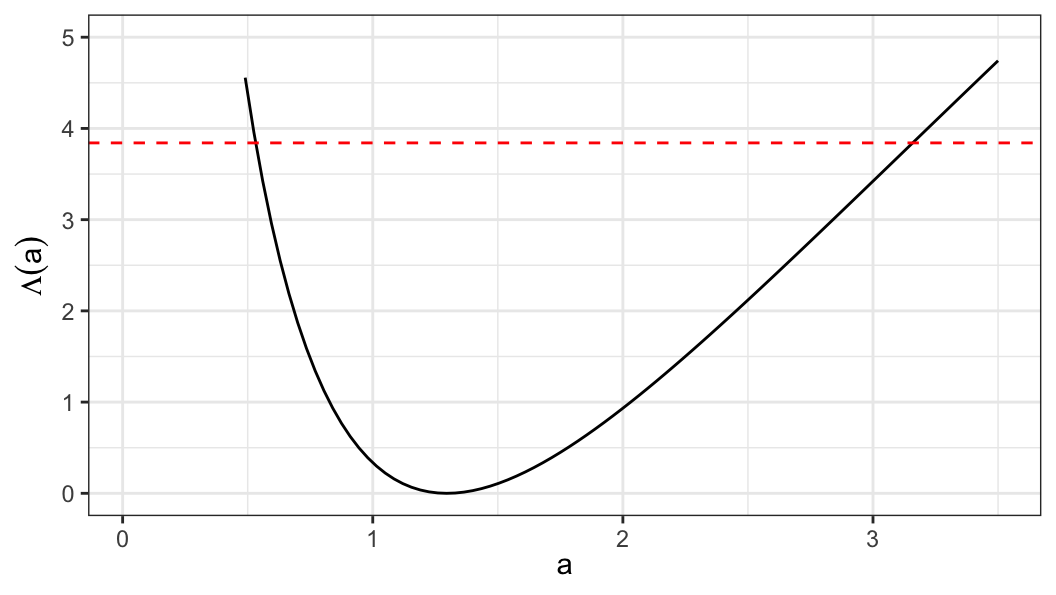
- 95% of \((\theta_1/\theta_2)\) is the range of values of \(a=(\theta_1/\theta_2)\), such that \[ \Lambda(a) \leq \chi^2_{(1), .95} = 3.84 \] which is \[ 0.56 < a < 3.15\;\;\Rightarrow\;\;0.56 < (\theta_1/\theta_2) < 3.15 \]
| method | lower | upper |
|---|---|---|
| Normal approximation | 0.54 | 3.114 |
| LRT | 0.56 | 3.150 |
Type II censored sample (CI for \(\theta_1/\theta_2\))
Lifetime distributions \(T_{i}\sim \text{Exp}(\theta_i)\;i=1, 2\)
Type II censored sample for the group \(i\), which has \(r_i\) number of failures and \((n_i-r_i)\) subjects are censored at \(t_{(ir_i)}\) \[ t_{(i1)}<\cdots<t_{(ir_i)} \]
- Likelihood function \[ \begin{aligned} L(\theta_1, \theta_2) & = \prod_{i=1}^2 (1/\theta_i)^{r_i}\,e^{-\sum_jt_{(ij)}/\theta_i} \;\;e^{-(n_i-r_i)t_{(ir_i)}/\theta_i} \\ & = \prod_{i=1}^2 (1/\theta_i)^{r_i}\,e^{-(1/\theta_i)\big[\sum_jt_{(ij)}+(n_i-r_i)t_{(ir_i)}\big]} \\ & = \prod_{i=1}^2 (1/\theta_i)^{r_i}\,e^{-T_i/\theta_i} \end{aligned} \]
MLE \[ \hat\theta_i = \frac{T_i}{r_i} \]
We have already shown that \[ \frac{2T_i}{\theta_i} = \frac{2r_i\hat\theta_i}{\theta_i}\sim \chi_{(2r_i)}^2 \]
Then we can show \[ \frac{(2r_1\hat\theta_1/\theta_1)/(2r_1)}{(2r_2\hat\theta_2/\theta_2)/(2r_2)} = \frac{\hat\theta_1\theta_2}{\hat\theta_2\theta_1}\sim F_{(2r_1, 2r_2)} \]
We can write \[ P\Big(F_{(2r_1, 2r_2), \alpha/2} \leq \frac{\hat\theta_1\theta_2}{\hat\theta_2\theta_1} \leq F_{(2r_1, 2r_2), 1-\alpha/2} \Big) = 1-\alpha \]
\((1-\alpha)100\%\) confidence interval for \((\theta_1/\theta_2)\) \[\begin{align} \frac{(\hat\theta_1/\hat\theta_2)}{F_{(2r_1, 2r_2), 1-\alpha/2}} \leq (\theta_1/\theta_2) \leq \frac{(\hat\theta_1/\hat\theta_2)}{F_{(2r_1, 2r_2), \alpha/2}} \end{align}\]
References
Sprott, David Arthur. 1980. “Maximum Likelihood in Small Samples: Estimation in the Presence of Nuisance Parameters.” Biometrika 67 (3): 515–23.