Inference for location-scale distributions
Likelihood based methods
The goal is to estimate the parameters \((u,b)\) or \((\alpha,\beta)\)
For likelihood-based inference, estimating \((u,b)\) (or equivalently \((u,\log b)\)) has several advantages:
- the log-likelihood is typically closer to quadratic;
- normal approximations for \((\hat u,\hat b)\) tend to be more accurate;
- numerical optimization is more stable;
- most statistical software (e.g.,
survreg() in R) uses the \((u,\log b)\) parameterization.
In the following sections, likelihood-based inference procedures are developed using the \((u,b)\) parameterization, with results later transformed to \((\alpha,\beta)\) for interpretation on the original time scale.
Likelihood function
Suppose we observe a possibly right-censored sample \[
\{(t_i,\delta_i),\; i=1,\ldots,n\},
\] where \(t_i\) is the observed time and \(\delta_i=1\) indicates a failure while \(\delta_i=0\) indicates right censoring.
Define \[
y_i=\log t_i
\quad\text{and}\quad
z_i=\frac{y_i-u}{b}.
\]
For a log-location–scale model with standard survivor function \(S_0(\cdot)\) and density \(f_0(\cdot)\), the likelihood function is \[
L(u,b)
=\prod_{i=1}^n
\Bigg[\frac{1}{b}f_0(z_i)\Bigg]^{\delta_i}
\Big[S_0(z_i)\Big]^{1-\delta_i}.
\]
The corresponding log-likelihood function is \[
\ell(u,b) = -r\log b + \sum_{i=1}^n \Big[\delta_i\log f_0(z_i) + (1-\delta_i)\log S_0(z_i)\Big],
\] where \(r=\sum_{i=1}^n\delta_i\) is the total number of failures.
Score functions
\[
\begin{aligned}
{\color{purple} \ell(u, b)} & = {\color{purple} -r\log b +\sum_{i=1}^n\Big[\delta_i\log f_0(z_i) + (1-\delta_i)\log S_0(z_i)\Big] } \\
& = -r\log b + \sum_{i=1}^n\ell_i(z_i, \delta_i)
\end{aligned}
\]
\[
\begin{aligned}
\frac{\partial \ell(u, b)}{\partial u} &= \sum_{i=1}^n\frac{\partial \ell_i(z_i, \delta_i)}{\partial z_i}\times \frac{\partial z_i}{\partial u}\notag \\
&= \sum_{i=1}^n\frac{\partial \ell_i(z_i, \delta_i)}{\partial z_i}\times \bigg(\frac{-1}{b}\bigg)\notag\\[.5em]
& = -\frac{1}{b} \sum_{i=1}^n\bigg[\delta_i\,\frac{\partial \log f_0(z_i)}{\partial z_i} + (1-\delta_i)\, \frac{\partial \log S_0(z_i)}{\partial z_i}\bigg]\notag
\end{aligned}
\]
\[
{\color{purple} \ell(u, b) = -r\log b +\sum_{i=1}^n\Big[\delta_i\log f_0(z_i) + (1-\delta_i)\log S_0(z_i) \Big]}
\]
\[
\begin{aligned}
\frac{\partial \ell(u, b)}{\partial b} &= -\frac{r}{b} + \sum_{i=1}^n\frac{\partial \ell_i(z_i, \delta_i)}{\partial z_i}\times \frac{\partial z_i}{\partial b}\notag \\
&= -\frac{r}{b} + \sum_{i=1}^n \frac{\partial \ell_i(z_i, \delta_i)}{\partial z_i}\times \Bigg(\frac{-z_i}{b}\Bigg)\notag\\[.5em]
& = -\frac{r}{b} -\frac{1}{b} \sum_{i=1}^nz_i\bigg[\delta_i\,\frac{\partial \log f_0(z_i)}{\partial z_i} + (1-\delta_i)\, \frac{\partial \log S_0(z_i)}{\partial z_i}\bigg]\notag
\end{aligned}
\]
Hessian matrix
\[
{\color{purple} \frac{\partial \ell(u, b)}{\partial u} = -\frac{1}{b} \sum_{i=1}^n\bigg[\delta_i\,\frac{\partial \log f_0(z_i)}{\partial z_i} + (1-\delta_i)\, \frac{\partial \log S_0(z_i)}{\partial z_i}\bigg]}
\]
\[\begin{align*}
\frac{\partial^2 \ell(u, b)}{\partial u^2} & = \frac{\partial}{\partial u} \bigg[\frac{\partial \ell(u, b)}{\partial u}\bigg]\\[.35em] %& = \frac{\partial}{\partial %z_i}\bigg[\frac{\partial \ell(u, b)}{\partial u}\bigg]\; %\frac{\partial z_i}{\partial u}\notag \\[.35em]
& = \frac{1}{b^2} \sum_{i=1}^n\bigg[\delta_i\,\frac{\partial^2 \log f_0(z_i)}{\partial z_i^2} + (1-\delta_i)\, \frac{\partial^2 \log S_0(z_i)}{\partial z_i^2}\bigg]
\end{align*}\]
\[
{\color{purple}\frac{\partial \ell(u, b)}{\partial b} = -\frac{r}{b} -\frac{1}{b} \sum_{i=1}^nz_i\bigg[\delta_i\,\frac{\partial \log f_0(z_i)}{\partial z_i} + (1-\delta_i)\, \frac{\partial \log S_0(z_i)}{\partial z_i}\bigg]}
\]
\[\begin{align*}
\frac{\partial^2 \ell(u, b)}{\partial b^2} & = \frac{r}{b^2} +\frac{2}{b^2} \sum_{i=1}^nz_i\bigg[\delta_i\,\frac{\partial \log f_0(z_i)}{\partial z_i} + (1-\delta_i)\, \frac{\partial \log S_0(z_i)}{\partial z_i}\bigg]\\[.25em]
& \;\;\;+\frac{1}{b^2}\sum_{i=1}^nz_i^2\bigg[\delta_i\,\frac{\partial^2 \log f_0(z_i)}{\partial z_i^2} + (1-\delta_i)\, \frac{\partial^2 \log S_0(z_i)}{\partial z_i^2}\bigg]
\end{align*}\]
\[\begin{align*}
{\color{purple} \frac{\partial \ell(u, b)}{\partial u}} &= {\color{purple}-\frac{1}{b} \sum_{i=1}^n\bigg[\delta_i\,\frac{\partial \log f_0(z_i)}{\partial z_i} + (1-\delta_i)\, \frac{\partial \log S_0(z_i)}{\partial z_i}\bigg]} \\[.5em]
\frac{\partial^2 \ell(u, b)}{\partial u\,\partial b}
& = \frac{1}{b^2} \sum_{i=1}^n\bigg[\delta_i\,\frac{\partial \log f_0(z_i)}{\partial z_i} + (1-\delta_i)\, \frac{\partial \log S_0(z_i)}{\partial z_i}\bigg]\\[.25em]
&\;\; \;\;+ \frac{1}{b^2} \sum_{i=1}^nz_i\bigg[\delta_i\,\frac{\partial^2 \log f_0(z_i)}{\partial z_i^2} + (1-\delta_i)\, \frac{\partial^2 \log S_0(z_i)}{\partial z_i^2}\bigg]
\end{align*}\]
Statistical inference
The maximum likelihood estimator (MLE) of \((u,b)\) is defined as \[
(\hat u, \hat b)' = {\arg\,\max}_{(u, b)' \in \Theta} \ell(u, b).
\]
Under regularity conditions, the asymptotic covariance matrix of \((\hat u,\hat b)'\) can be estimated by the inverse of the observed information matrix evaluated at the MLEs: \[
\operatorname{Var}\!\begin{pmatrix}\hat u \\ \hat b\end{pmatrix}
\approx \hat V
= \Big[I(\hat u, \hat b)\Big]^{-1},
\]
Sampling distribution
\[
\begin{pmatrix}\hat u \\ \hat b\end{pmatrix} \sim \mathcal{N}_2\begin{pmatrix} \begin{bmatrix} u \\ b\end{bmatrix}, \Big[I(\hat u, \hat b)\Big]^{-1} \end{pmatrix}
\]
Wald type CIs
For a large \(n\), \((\hat u, \hat b)'\) follows a bivariate normal distribution with mean \((u, b)'\) and variance matrix \(\hat V\)
Standard error of \(\hat u\) and \(\hat b\) can be obtained from the diagonal elements of \(\hat V\) \[
se(\hat u) = \hat{V}_{11}^{1/2}\;\;\text{and}\;\;se(\hat b) = \hat{V}_{22}^{1/2}
\]
-
Following pivotal quantities follow standard normal distributions \[
\begin{aligned}
Z_1 = \frac{\hat u - u}{se(\hat u)},\;\; \;\;\;
Z_2 = \frac{\hat b - b}{se(\hat b)}, \;\;\;\;\;
Z_2' = \frac{\log \hat b - \log b}{se(\log \hat b)}
\end{aligned}
\]
- \(se(\log \hat b) = se(\hat b)/\hat b\)
\((1-p)100\%\) confidence intervals \[
\begin{aligned}
\hat u &\pm z_{1-p/2}\,se(\hat u) \\
\hat b &\pm z_{1-p/2}\,se(\hat b) \\
\hat b &\exp\{\pm z_{1-p/2}\,se(\log \hat b)\}
\end{aligned}
\]
Likelihood ratio test based CI
Normal approximation based confidence intervals could be inaccurate for small samples
An alternative to normal approximation, bootstrap simulations can be used to estimate the distributions of pivots
All these methods can perform poorly in small samples with heavy censoring
Implementation of likelihood ratio based confidence intervals is relatively complicated, but LRT based CI often performs better in small and medium-size samples
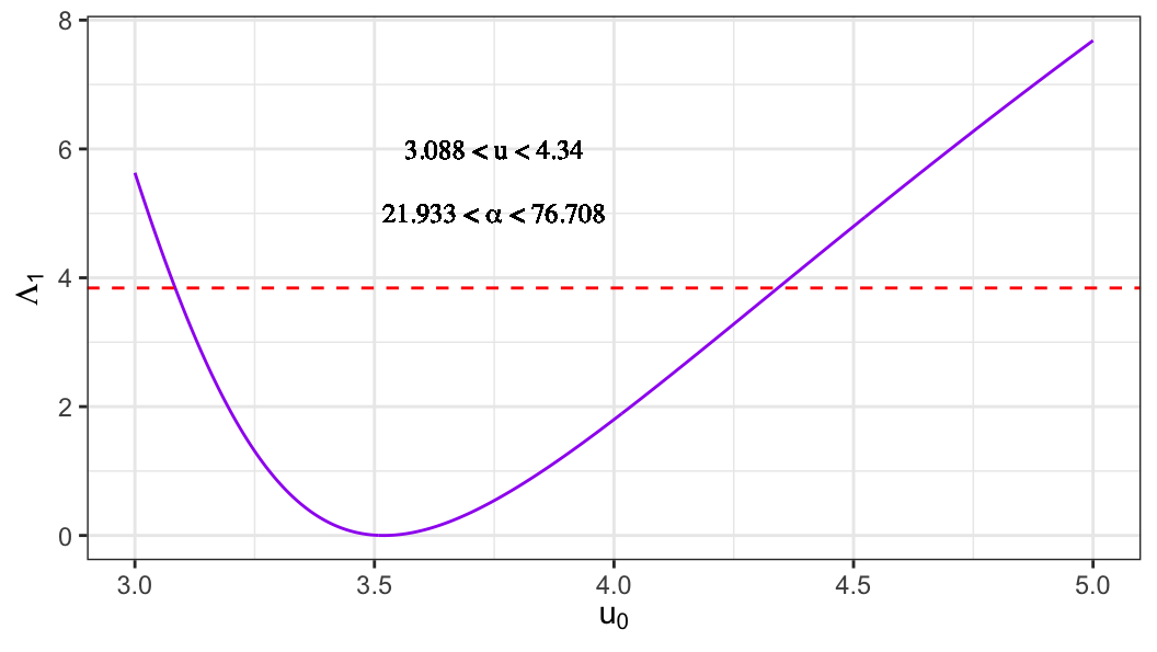
LRT-based CI for the location parameter \(u\)
To test the null hypothesis \(H_0: u = u_0\), the likelihood ratio test statistic is \[
\Lambda_1(u_0)
= 2\ell(\hat u, \hat b)
- 2\ell(u_0, \tilde b(u_0)),
\] where \[
\begin{aligned}
(\hat u, \hat b)'
&= {\arg\,\max}_{(u, b)' \in \Theta} \ell(u, b),
\qquad \text{(unrestricted MLEs)}, \\
\tilde b(u_0)
&= {\arg\,\max}_{b \in \Theta} \ell(u_0, b),
\qquad \text{(MLE under } H_0\text{)}.
\end{aligned}
\]
Under \(H_0\), \[
\Lambda_1(u_0) \xrightarrow{d} \chi^2_{(1)}.
\]
An approximate two-sided \(100(1-p)\%\) confidence interval for \(u\) is given by the set of values \(u_0\) such that \[
\Lambda_1(u_0) \leq \chi^2_{(1),\,1-p}.
\]
Homework
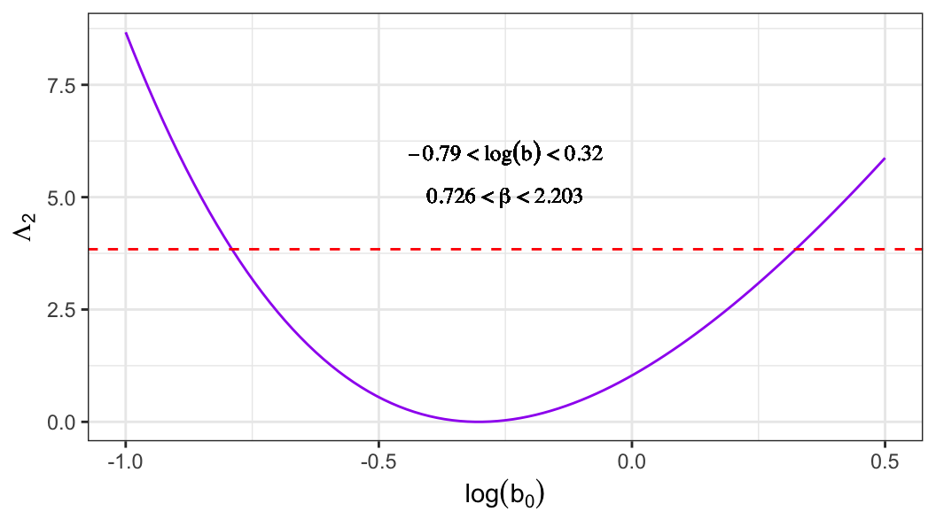
- Derive the likelihood ratio test–based confidence interval for the scale parameter \(b\).
Quantiles and their confidence intervals
Quantiles of log-lifetime
The \(p\)th quantile of the log-lifetime variable \(Y\) satisfies \[
P(Y \le y_p) = p.
\]
Equivalently, \[
S_0\!\left(\frac{y_p-u}{b}\right)=1-p,
\] which implies \[
y_p = u + b w_p,
\qquad
w_p = S_0^{-1}(1-p)=F_0^{-1}(p).
\]
Wald-type CI for \(y_p\)
An estimator of \(y_p\) is \[
\hat y_p = \hat u + \hat b w_p.
\]
Using the delta method, its standard error is \[
se(\hat y_p) = \sqrt{\hat V_{11} + w_p^2 \hat V_{22} + 2w_p \hat V_{12}}.
\]
The pivotal quantity \[
Z_p = \frac{\hat y_p - y_p}{se(\hat y_p)}
\] is approximately standard normal, leading to a \(100(1-q)\%\) confidence interval \[
\hat y_p \pm z_{1-q/2}\,se(\hat y_p).
\]
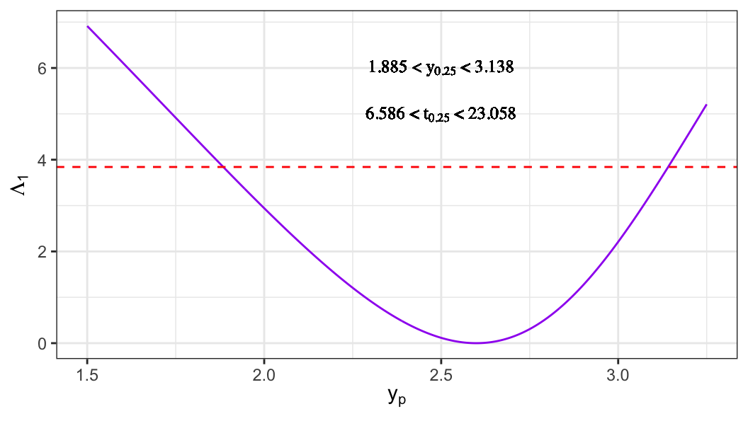
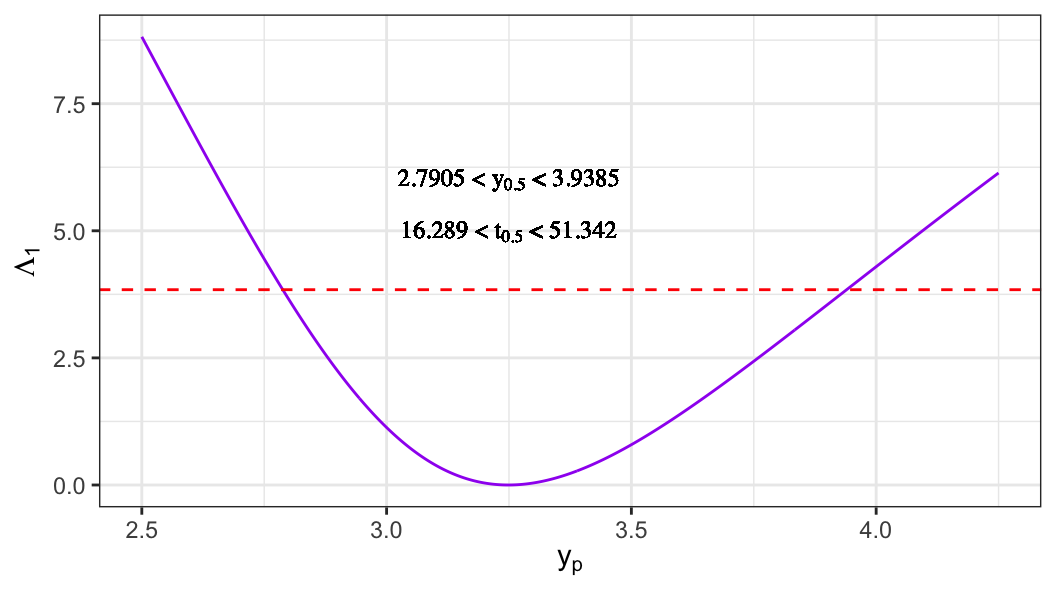
LRT-based CI for quantiles
The \(p\)th quantile can be expressed as \[
y_p = u + w_p b.
\]
To obtain an LRT-based confidence interval for \(y_p\), consider the null hypothesis \[
H_0: y_p = y_{p_0}.
\]
The likelihood ratio statistic is \[
\Lambda(y_{p_0})
= 2\ell(\hat u, \hat b)
- 2\ell(\tilde u, \tilde b),
\tag{5.1}\] where \((\tilde u,\tilde b)\) are the MLEs under \(H_0\).
Steps to compute \((\tilde u,\tilde b)\)
- Under \(H_0\), \(u = y_{p_0} - w_p b\).
- Obtain \[
\tilde b
= {\arg\,\max}_{b\in\Theta}
\ell(y_{p_0}-w_pb,\,b).
\]
- Set \[
\tilde u = y_{p_0} - w_p \tilde b.
\]
An approximate \(100(1-q)\%\) confidence interval for \(y_p\) is given by the set of \(y_{p_0}\) values satisfying \[
\Lambda(y_{p_0}) \le \chi^2_{(1),\,1-q}.
\]
The general likelihood results developed above apply to all log-location–scale models.
In the following sections, these results are specialized to particular distributions, beginning with the extreme-value and Weibull models.